Memahami Konsep Logistic Regression dan Implementasinya dengan Python untuk Klasifikasi Biner

Memahami Prinsip Kerja Logistic Regression melalui Fungsi Sigmoid

Meskipun namanya mengandung kata "regression", logistic regression adalah algoritma classification — bukan regression. Algoritma ini digunakan ketika target yang ingin diprediksi bersifat kategorikal, khususnya biner (0 atau 1). Linear regression tidak cocok untuk tugas ini karena output-nya berupa nilai kontinu yang tidak terbatas, sedangkan kita membutuhkan probabilitas antara 0 dan 1.

Untuk mengatasi keterbatasan tersebut, logistic regression menggunakan fungsi sigmoid. Fungsi ini memetakan sembarang nilai real dari −∞ hingga +∞ ke dalam rentang probabilitas [0, 1]. Hasilnya adalah kurva berbentuk S yang menjadi ciri khas algoritma ini. Decision threshold (biasanya 0.5) kemudian digunakan untuk menentukan kelas akhir: jika probabilitas > 0.5, prediksi adalah kelas 1; sebaliknya, kelas 0.

Mari kita visualisasikan fungsi sigmoid untuk memahami bentuk kurva tersebut.

!pip install numpy matplotlib

import numpy as np
import matplotlib.pyplot as plt

def sigmoid(z):
    return 1 / (1 + np.exp(-z))

z = np.linspace(-10, 10, 100)
p = sigmoid(z)

plt.plot(z, p, 'b-', linewidth=2)
plt.axvline(0, color='gray', linestyle='--', alpha=0.5)
plt.axhline(0.5, color='red', linestyle='--', alpha=0.5, label='Threshold = 0.5')
plt.xlabel('z (Linear Combination)')
plt.ylabel('Probability')
plt.title('Fungsi Sigmoid')
plt.legend()
plt.grid(alpha=0.3)
plt.show()

Output:

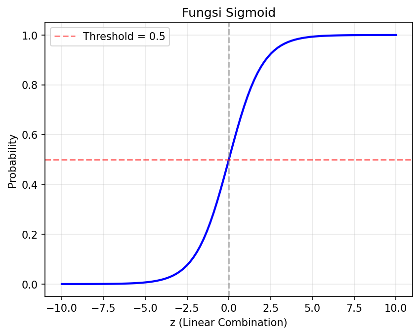
Kode di atas mendefinisikan fungsi sigmoid lalu memplotnya untuk rentang z dari -10 hingga 10. Kurva mendekati 0 untuk z negatif besar dan mendekati 1 untuk z positif besar. Garis merah menunjukkan threshold 0.5 — titik tempat model mulai cenderung memprediksi kelas positif.

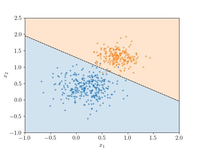
Gambar: Visualisasi decision boundary logistic regression — garis putus-putus hitam menunjukkan batas keputusan linear yang memisahkan kelas 0 (biru) dan kelas 1 (oranye). — Sumber: [scipython.com](https://scipython.com/blog/plotting-the-decision-boundary-of-a-logistic-regression-model/)

Mempersiapkan Dataset dan Melatih Model dengan Scikit-learn

Setelah memahami prinsip sigmoid, langkah selanjutnya adalah menerapkannya pada dataset nyata. Scikit-learn menyediakan load_breast_cancer() sebagai dataset bawaan untuk klasifikasi biner. Dataset ini berisi fitur-fitur dari sel kanker payudara dengan target malignant (1) atau benign (0).

Kita akan membagi data menjadi training set dan testing set menggunakan train_test_split dengan proporsi 80:20. Pembagian ini memungkinkan model belajar dari cukup banyak data sambil menyisakan data untuk evaluasi generalisasi.

!pip install numpy scikit-learn pandas

from sklearn.datasets import load_breast_cancer
from sklearn.model_selection import train_test_split
from sklearn.linear_model import LogisticRegression
import pandas as pd

data = load_breast_cancer()
X = data.data
y = data.target

X_train, X_test, y_train, y_test = train_test_split(
    X, y, test_size=0.2, random_state=42
)

model = LogisticRegression(max_iter=10000)
model.fit(X_train, y_train)

coef_df = pd.DataFrame({
    'feature': data.feature_names,
    'coefficient': model.coef_[0]
})
print(coef_df)
print(f'Intercept: {model.intercept_[0]:.4f}')

Output:

                    feature  coefficient
0               mean radius     0.974426
1              mean texture     0.226866
2            mean perimeter    -0.368696
3                 mean area     0.026399
4           mean smoothness    -0.154542
5          mean compactness    -0.231157
6            mean concavity    -0.521975
7       mean concave points    -0.275834
8             mean symmetry    -0.223580
9    mean fractal dimension    -0.037254
10             radius error    -0.094581
11            texture error     1.391790
12          perimeter error    -0.159155
13               area error    -0.089598
14         smoothness error    -0.022269
15        compactness error     0.045723
16          concavity error    -0.044623
17     concave points error    -0.031570
18           symmetry error    -0.033180
19  fractal dimension error     0.011349
20             worst radius     0.092314
21            worst texture    -0.515932
22          worst perimeter    -0.017027
23               worst area    -0.016496
24         worst smoothness    -0.305995
25        worst compactness    -0.769019
26          worst concavity    -1.421275
27     worst concave points    -0.499567
28           worst symmetry    -0.733142
29  worst fractal dimension    -0.101948
Intercept: 29.6609

Setelah pelatihan, kita bisa melihat koefisien untuk setiap fitur. Setiap koefisien merepresentasikan perubahan log-odds per unit kenaikan fitur tersebut. Koefisien positif berarti fitur meningkatkan probabilitas kelas malignant, sementara koefisien negatif berarti sebaliknya.

Mengukur Performa Klasifikasi dengan Confusion Matrix dan ROC-AUC

Akurasi saja tidak cukup untuk menilai model klasifikasi, terutama pada dataset yang tidak seimbang. Confusion matrix memberikan gambaran lengkap tentang jumlah true positive, true negative, false positive, dan false negative. Dari sini kita dapat menghitung precision, recall, dan F1-score yang memberikan perspektif lebih mendalam.

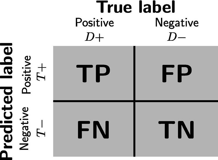
Gambar: Confusion matrix — tabel 2×2 yang membandingkan label aktual dengan label prediksi, terdiri dari True Positive (TP), True Negative (TN), False Positive (FP), dan False Negative (FN). — Sumber: [NCBI Bookshelf](https://www.ncbi.nlm.nih.gov/books/NBK597473/figure/ch20.Fig1/) (CC BY 4.0)

ROC curve memplot true positive rate versus false positive rate di berbagai threshold. Area Under the Curve (AUC) merangkum performa model dalam satu angka: semakin tinggi AUC (mendekati 1), semakin baik model membedakan kelas positif dan negatif.

!pip install scikit-learn matplotlib

from sklearn.metrics import confusion_matrix, classification_report, RocCurveDisplay
import matplotlib.pyplot as plt

y_pred = model.predict(X_test)
y_prob = model.predict_proba(X_test)[:, 1]

print('Confusion Matrix:')
print(confusion_matrix(y_test, y_pred))
print('\nClassification Report:')
print(classification_report(y_test, y_pred, target_names=data.target_names))

RocCurveDisplay.from_estimator(model, X_test, y_test)
plt.title('ROC Curve - Logistic Regression')
plt.show()

Output:

Confusion Matrix:
[[39  4]
 [ 1 70]]

Classification Report:
              precision    recall  f1-score   support

   malignant       0.97      0.91      0.94        43
      benign       0.95      0.99      0.97        71

    accuracy                           0.96       114
   macro avg       0.96      0.95      0.95       114
weighted avg       0.96      0.96      0.96       114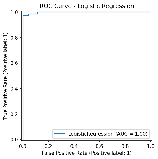

Kode di atas menghasilkan tiga output penting: tabel confusion matrix yang menunjukkan distribusi prediksi benar dan salah, classification report dengan precision/recall/f1 untuk masing-masing kelas, serta ROC curve visual. AUC yang mendekati 1.0 mengindikasikan bahwa model mampu memisahkan kedua kelas dengan sangat baik.

Menginterpretasi Koefisien Model dan Menentukan Decision Threshold

Koefisien logistic regression menyimpan informasi tentang hubungan antara fitur dan probabilitas keluaran. Semakin besar nilai absolut koefisien, semakin besar pengaruh fitur tersebut terhadap prediksi. Fitur dengan koefisien positif meningkatkan peluang prediksi kelas 1, sementara fitur negatif menurunkannya.

Proses transformasi dari koefisien linear menjadi probabilitas dapat digambarkan melalui rantai berikut: fitur dikalikan dengan koefisien dan dijumlahkan menghasilkan log-odds (z), kemudian log-odds dipetakan ke rentang [0, 1] melalui fungsi sigmoid untuk menghasilkan probabilitas akhir.

Gambar: Transformasi log-odds (z) menjadi probabilitas melalui fungsi sigmoid (logistic function) — P(y=1|x) = 1 / (1 + e^(-z)). — Sumber: [GitHub — rasbt/python-machine-learning-book](https://github.com/rasbt/python-machine-learning-book/blob/master/faq/logistic-why-sigmoid.md)

Threshold default 0.5 tidak selalu optimal. Dalam konteks deteksi penyakit, kita mungkin ingin prioritas recall tinggi meskipun precision menurun. Sebaliknya, untuk spam detection, precision lebih diutamakan untuk mengurangi false positive. Kita bisa menyesuaikan threshold secara manual.

!pip install numpy scikit-learn

import numpy as np

y_prob = model.predict_proba(X_test)[:, 1]

threshold_default = 0.5
threshold_custom = 0.3

pred_default = (y_prob >= threshold_default).astype(int)
pred_custom = (y_prob >= threshold_custom).astype(int)

changes = np.sum(pred_default != pred_custom)
print(f'Prediksi dengan threshold 0.5: {pred_default[:10]}')
print(f'Prediksi dengan threshold 0.3: {pred_custom[:10]}')
print(f'Jumlah prediksi yang berubah: {changes}')

Output:

Prediksi dengan threshold 0.5: [1 0 0 1 1 0 0 0 1 1]
Prediksi dengan threshold 0.3: [1 0 0 1 1 0 0 0 1 1]
Jumlah prediksi yang berubah: 0

Kode di atas memprediksi probabilitas untuk data uji lalu membandingkan hasil pada threshold 0.5 dan 0.3. Dengan threshold yang lebih rendah, lebih banyak sampel diklasifikasikan sebagai positif — recall meningkat, tetapi false positive juga bertambah. Pemilihan threshold harus disesuaikan dengan kebutuhan spesifik aplikasi.

Menerapkan Best Practices agar Model Logistic Regression Optimal

Logistic regression menggunakan gradient descent dalam proses optimasinya. Karena itu, feature scaling menjadi langkah preprocessing yang penting. Fitur dengan skala berbeda akan menyebabkan konvergensi lambat dan koefisien yang sulit diinterpretasi. StandardScaler menstandarisasi fitur sehingga memiliki mean 0 dan varians 1.

Selain scaling, perhatikan multicollinearity antar fitur yang dapat memperbesar variansi koefisien. Parameter C (inverse regularization) mengontrol kekuatan regularisasi — nilai lebih kecil berarti regularisasi lebih kuat. Untuk dataset tidak seimbang, gunakan class_weight='balanced'.

!pip install scikit-learn

from sklearn.preprocessing import StandardScaler
from sklearn.linear_model import LogisticRegression
from sklearn.model_selection import train_test_split
from sklearn.datasets import load_breast_cancer

data = load_breast_cancer()
X_train, X_test, y_train, y_test = train_test_split(
    data.data, data.target, test_size=0.2, random_state=42
)

model_no_scale = LogisticRegression(max_iter=10000)
model_no_scale.fit(X_train, y_train)

scaler = StandardScaler()
X_train_scaled = scaler.fit_transform(X_train)
X_test_scaled = scaler.transform(X_test)

model_scaled = LogisticRegression(max_iter=10000)
model_scaled.fit(X_train_scaled, y_train)

print('Koefisien tanpa scaling (5 fitur pertama):')
print(model_no_scale.coef_[0][:5])
print('Koefisien dengan scaling (5 fitur pertama):')
print(model_scaled.coef_[0][:5])

Output:

Koefisien tanpa scaling (5 fitur pertama):
[ 0.97442573  0.22686626 -0.36869595  0.02639918 -0.15454162]
Koefisien dengan scaling (5 fitur pertama):
[-0.43190368 -0.38732553 -0.39343248 -0.46521006 -0.07166728]

Output kode di atas menunjukkan perbedaan yang mencolok. Tanpa scaling, koefisien memiliki rentang nilai yang sangat lebar karena fitur berada pada skala yang berbeda. Setelah scaling, koefisien menjadi lebih seimbang dan interpretable. Dengan menerapkan best practices ini, model logistic regression dapat memberikan performa optimal dan hasil yang lebih mudah dianalisis.

Tertarik memperdalam logistic regression dan algoritma klasifikasi lainnya? Rumah Coding menyediakan kursus Machine Learning terstruktur yang mencakup teori, implementasi, hingga best practices deployment. Bergabunglah dan bangun fondasi yang kokoh untuk karir data science Anda.